Hacking

Florian Ziemen

Tobias Kölling

Lukas Kluft

2025-05-12

Have fun
and
learn about Earth

Smooth workflows for km-scale data

(Code)

Made possible by

Loading less data

Load only the data you need

Both plots have the same number of pixels.

You should load the same amount of data to make them.

Our approach

• HEALPix Grid
• Resolution hierarchies
• Chunked storage (you’ll probably not see much of this)
• Catalogs grouping the datasets

HEALPix

• Hierarchical
• Equal Area
• isoLatitude

Pixelation

Górski et al., 2004

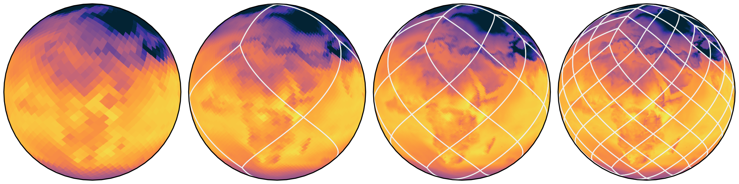
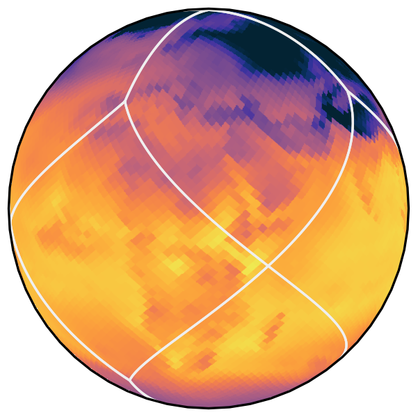
HEALPix features

• Uniform coverage of Earth
• Direct translation between lat/lon and pixel ID
• Cells arranged in isolatitude bands
• Index is a space-filling curve

Healpix hierarchy

Refinement by splitting each cell into four finer cells

Load only the data you need

• Global mean -> Level 0 (12 cells)
• Test a global map -> Level 5 (12288 cells)
• Fill a screen -> Level 9 (3M cells)
• Analyze a detail -> load only the region

Catalogs and phone books

• Basically your phone’s list of contacts
• You ask for a name, it will call the dataset
• Update it when the phone number of your contact changes
• No update needed when your contact gets a new phone
• share it in the team, and save effort updating

Catalogs

• Call it by its name, not by the location

  cat["casesm2_10km_cumulus"].to_dask()

  instead of

  xr.open_dataset("/lustre/persons_name/experiments/attempt7/outdata/data_*_74_b.nc")

• No need to know where data is.

• Parameterize variants

  cat["casesm2_10km_cumulus"](zoom=5, time="PT3H")

Let’s get real

Working with the catalog

Index generated from the catalog

https://digital-earths-global-hackathon.github.io/catalog/

Locations and datasets

• Our catalog has two dimensions
  • Location
  • Dataset
• Any dataset can be hosted at different locations
• Online datasets are availabe at all locations
• Local copies are preferred

Load the catalog

import intake
cat_url = "https://digital-earths-global-hackathon.github.io/catalog/catalog.yaml"
node = "CN"
cat = intake.open_catalog(cat_url)[node]

Get the phone number of a dataset

name = "casesm2_10km_cumulus"
cat[name].urlpath

'/data2/share/florain/CAS-ESM2_10km_cumulus_3d6h_z9.zarr'

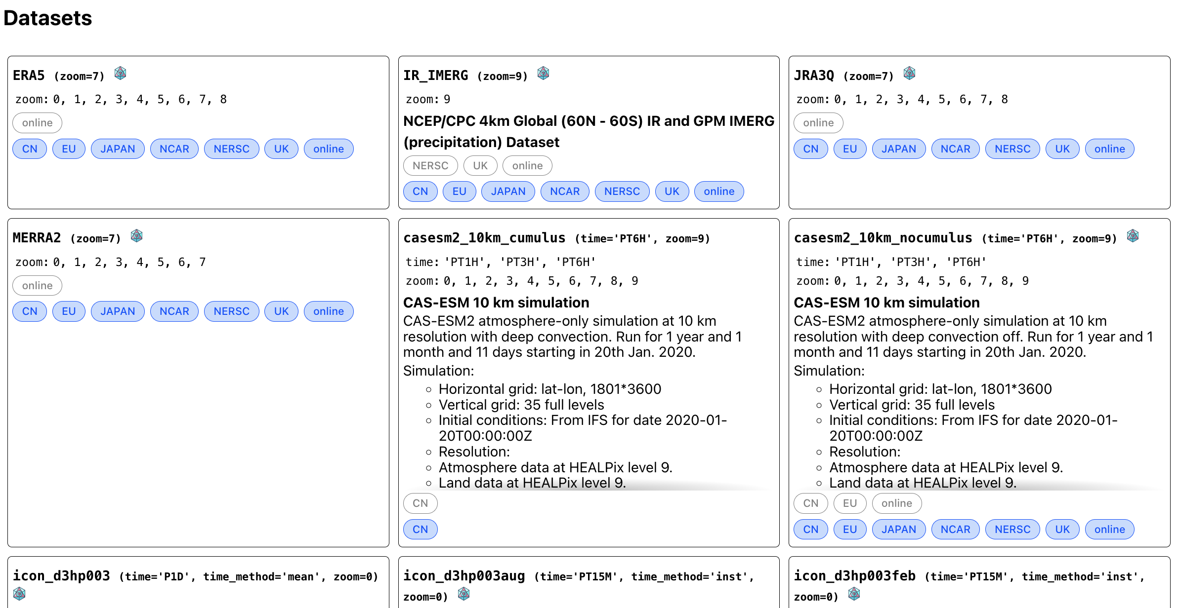
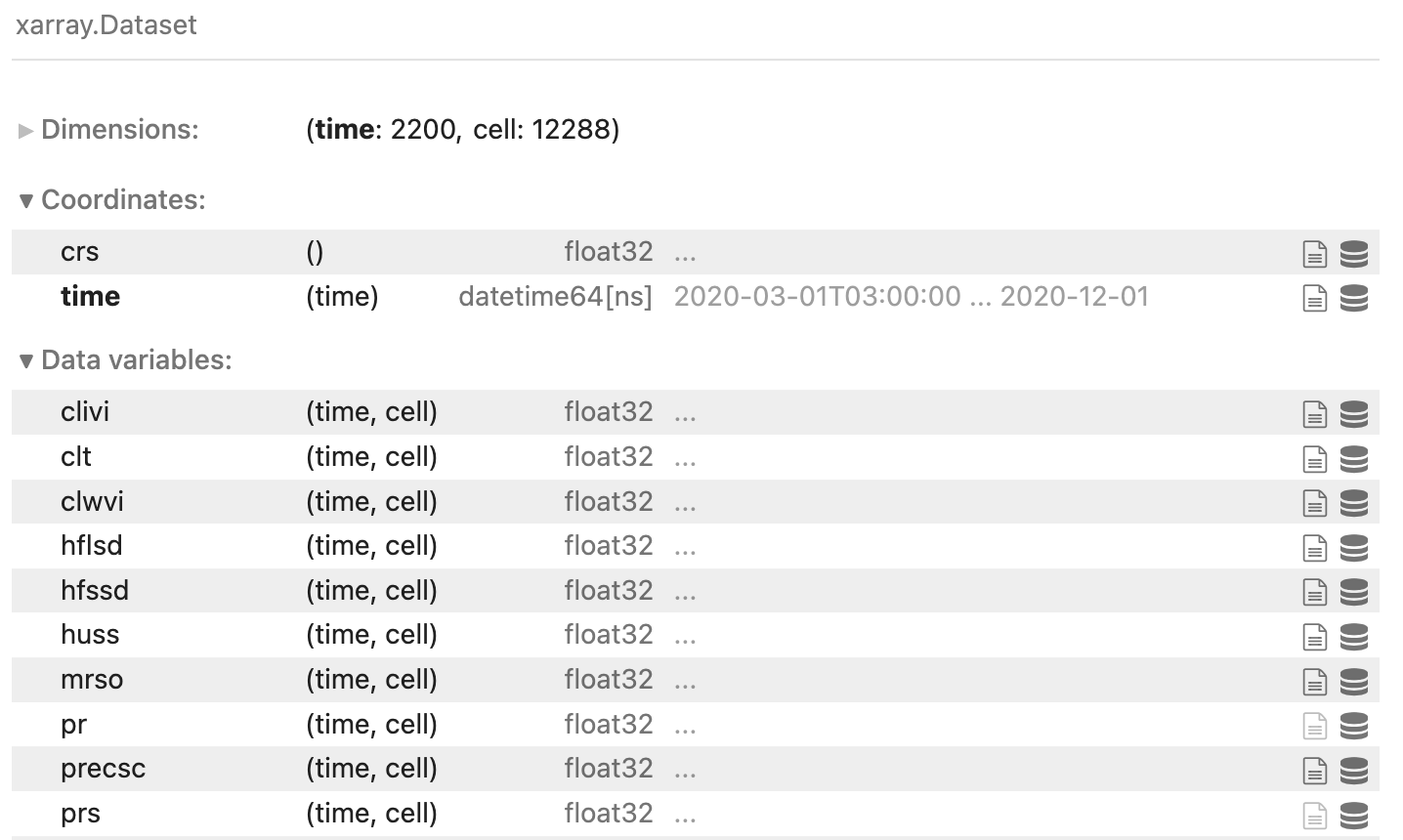
Call the dataset directly

cat[name].to_dask()

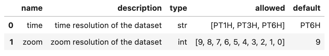
Look at the possible parameters

import pandas as pd
pd.DataFrame(cat[name].describe()['user_parameters'])

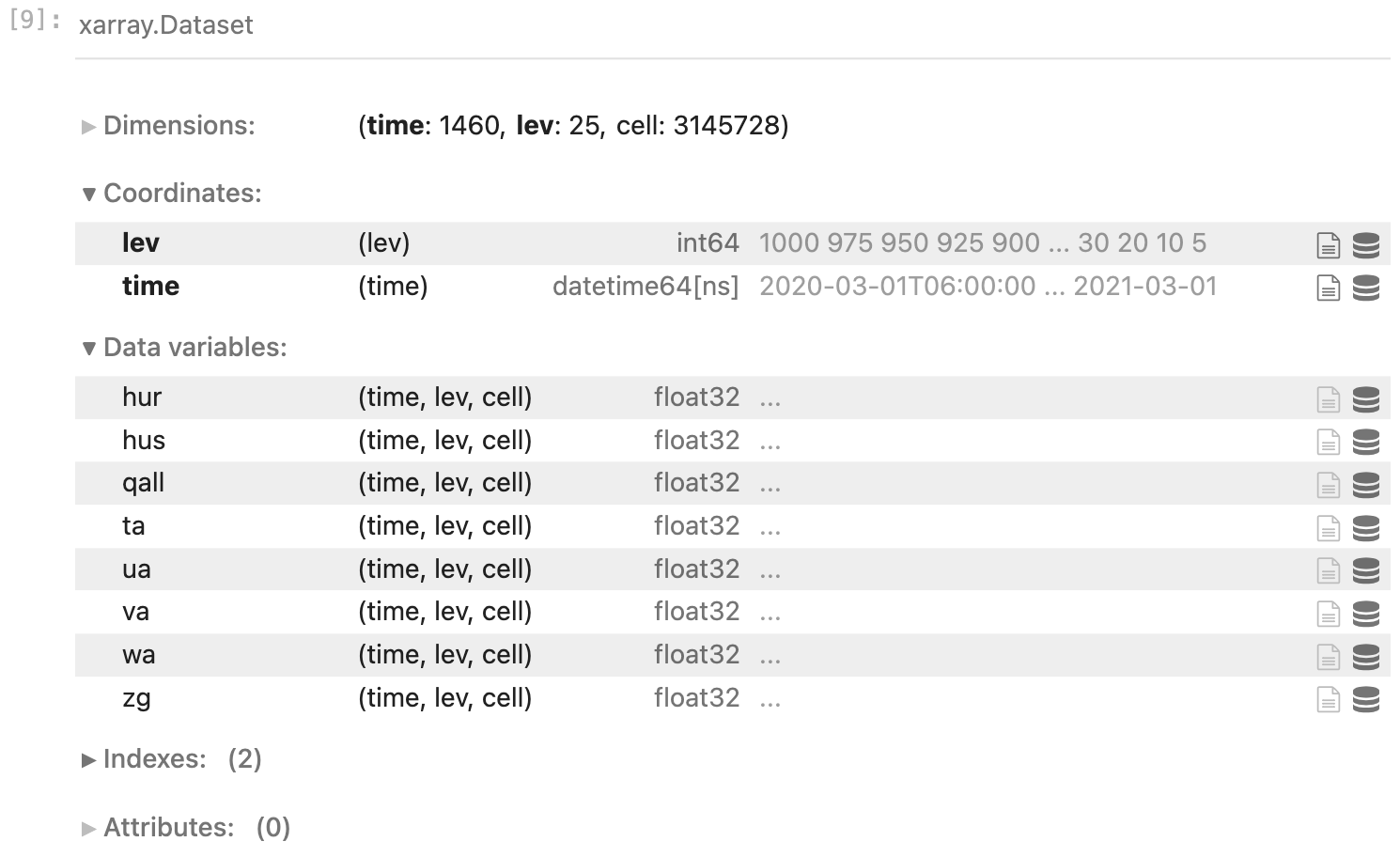
Load a specific variant

ds = cat[name](zoom=5, time="PT3H").to_dask()
ds

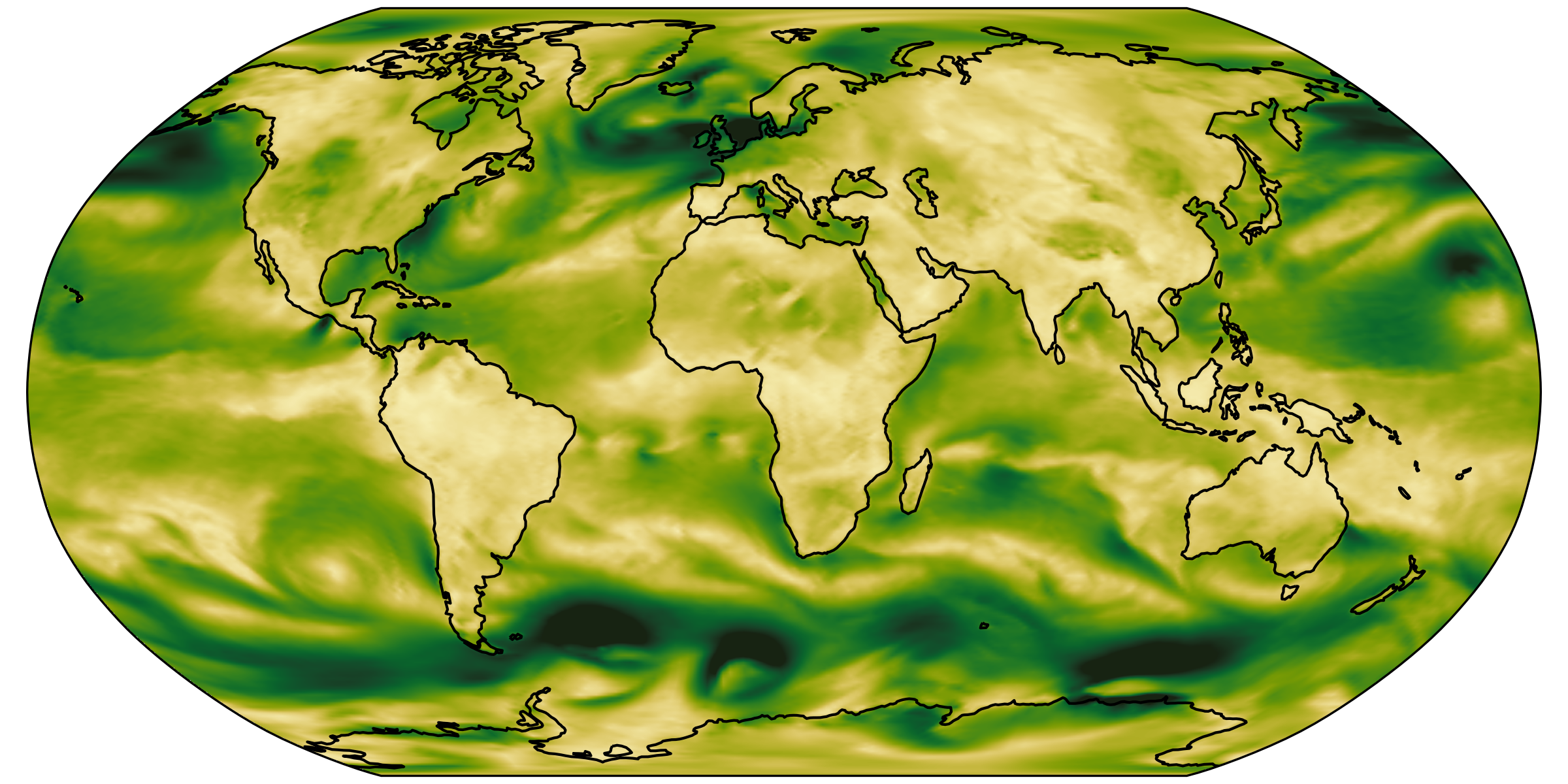
# Mapmaking

A simple world map

import easygems.healpix as egh
var = "tas"
plot_time = "2020-05-12T09:00:00"
cmap = "inferno"
egh.healpix_show(ds[var].sel(time=plot_time), cmap=cmap) 

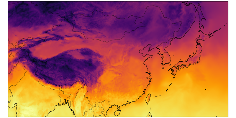
increasing the resolution

ds = cat[name](zoom=7, time="PT3H").to_dask()
egh.healpix_show(ds[var].sel(time=plot_time), cmap=cmap)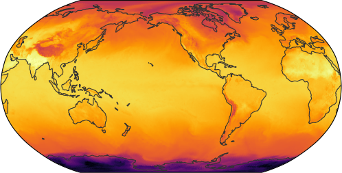 

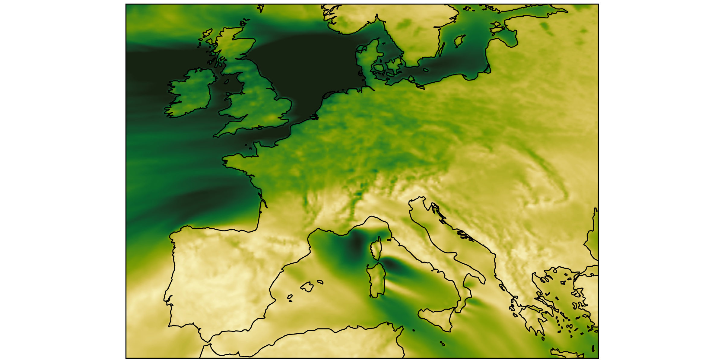
Zooming in

import cartopy.crs as ccrs
import cartopy.feature as cf

ds = cat[name](zoom=9, time="PT3H").to_dask()
projection = ccrs.Robinson(central_longitude=120)
fig, ax = plt.subplots(
  figsize=(8, 4), 
  subplot_kw={"projection": projection}, 
  constrained_layout=True
)
ax.set_extent([70, 150, 18, 55], crs=ccrs.PlateCarree())
egh.healpix_show(ds.tas.isel(time=0), 
  ax=ax, 
  cmap=cmap)
ax.add_feature(cf.COASTLINE, linewidth=0.8)
ax.add_feature(cf.BORDERS, linewidth=0.4)

Zooming in

More map examples on easy.gems

https://easy.gems.dkrz.de/Processing/healpix/healpix_cartopy.html

Zonal means

ds = cat[name](zoom=5, time="PT3H").to_dask().pipe(egh.attach_coords)
pr = ds['pr'].mean(dim='time').groupby(ds.lat).mean()
pr.plot()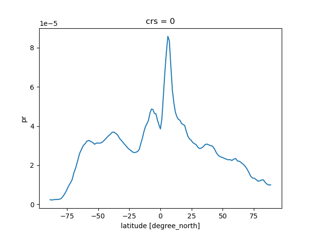

Zonal section

import matplotlib.pyplot as plt
ds = cat[name](zoom=5, time="PT6H").to_dask().pipe(egh.attach_coords)
ua = ds['ua'].mean(dim='time').groupby(ds.lat).mean()
ua.plot()
plt.ylim(plt.ylim()[::-1])
plt.title (f"Zonal mean zonal wind speed (m/s)")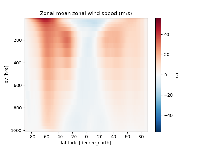

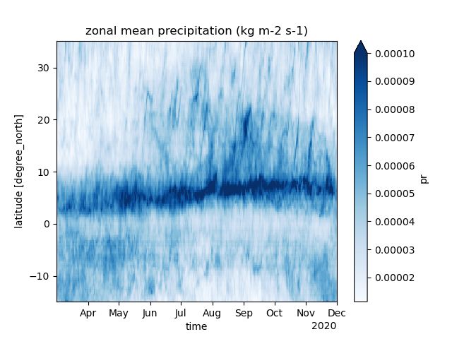
Space-time diagram

ds = cat[name](zoom=7, time="PT3H").to_dask().pipe(egh.attach_coords)
Slim, Nlim = -15.0, 35.0
pr = (
    ds['pr']
    .where((ds["lat"] > Slim) & (ds["lat"] < Nlim), drop=True)
    .groupby("lat")
    .mean()
).coarsen(time=8).mean().transpose().compute()
pr.plot(cmap="Blues", vmax=0.0001)
plt.title(f"zonal mean precipitation (kg m-2 s-1)")

More on time-space diagrams

https://easy.gems.dkrz.de/Processing/healpix/time-space.html

黑客马拉松圆满成功

A few words on datasets and Catalogs

Build clean datasets

• All variables together that fit together
• Cutting parts out is easier than gluing together
• Time spent on making them clean is saved during analysis
• Variants for coarsening should follow a logic

Catalogs arrange datasets logically

• Group dataset by topic
• Tree-Style catalogs allow for nesting
• Try to have exactly one catalog with good location
• Catalogs can be nested